Section 1 - The Maximum Flow Problem

Section 11B.1.1 The Maximum Flow Problem

The maximum flow problem seeks to produce the largest flow of fluid, electrons, signal --whatever -- between two points in a network (aka graph). The starting assumptions are that only some vertices on the graph have connections (edges) between them, and each edge has a maximum possible flow value (the "capacity" of that edge). Also, we have to specify a starting and ending vertex for the flow, the source and sink. So as not to use terminology that clashes with our source/destination terminology of edges, we will call the special vertices start and end.

The problem and algorithms work for all sorts of graphs, both directed and non-directed. To simplify our discussion we can confine our discussion to directed graphs (although the graphs do not have to be acyclic: i.e., they can contain cycles).

Here is a solved maximum flow problem with start vertex s and end vertex t. The input graph is on the left, and the maximum flow solution is on the right:

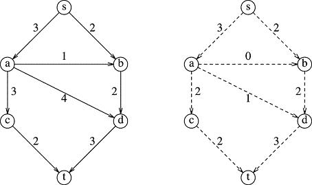
The way to interpret this is that for the pipe from s to a, i.e., edge (s, a), on the left graph, the maximum capacity that can be sustained is 3 (3 what? Mbits/second, gallons/minute, amperes, ... you name it). This is how all numbers on the left are interpreted: as the maximum capacities that each edge can handle. In order to get the maximum flow from s to t, we will find that we should send out the "stuff" according to the flow values on the right. Thus, we see we "max out" some pipes, but not all of them: edge (a, d) only carries 1 unit per time interval (its "flow") while it has a capacity of 4.

The question, of course, is: how do we arrive at the flow on the right in a systematic way, and how do we know it is really maximum?

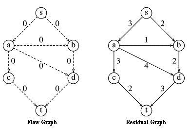
There are many maximum flow algorithms in use. Ours is not the fastest or most general, but it gets the job done and it is very easy. We start with two working graphs: They are both identical to the input graph except, possibly, for the edge costs. The first is the flow graph and it will start off with all edges having 0 capacity (cost 0). When the algorithm terminates, this will have the maximum flow values - it will be the solution. The second graph is called the residual graph and it starts out with the same edge costs as the input graph. These costs represent the unused potential flow that is still left to give to the algorithm. Initially, anything is possible up to the pipe capacities, because we have not chosen a particular path yet. As we start to commit ourselves to certain paths, we will use up some of that potential leaving less and less to work with as the algorithm progresses. The values will diminish as some of the potential flow in the residual graph is realized as actual flow in the flow graph. Therefore, the numbers will shift, gradually, from the residual graph to the flow graph until we have maxed out the capacity of so many flow graph edges that the flow graph will not support any further flow. At that point the algorithm will halt.

Here is a picture of the flow graph and residual graph at the start of the algorithm.

Section 11B.1.2 Reverse Flow in the Residual Graph

In fact, we will initialize our residual graph in a slightly different manner than shown above. It will be functionally the same, but the revision will make the algorithm work correctly. For each edge that we are given by the input graph, we will add an edge in the reverse direction with cost 0. Doing this does not really change the meaning of the residual graph since an edge with cost 0 can't be used to get anywhere, but you will see that these edges come into play as the algorithm progresses. Here is a portion of the correctly initialized residual graph with this modification:

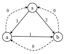
The purpose of these reverse flow edges (only added to the residual graph, not the flow graph, remember) is to allow us to "change our mind" as we make choices during the algorithm. For example, let's say we choose to send 2 units of flow from s to a during the algorithm. We would then have used up 2 of the 3 units of potential flow, and this would leave only 1 unit of residual flow for future use (inside the algorithm). The residual graph would reflect this reduced cost by revising (s, a) from 3 to 1. However, just in case we guessed wrong about this choice, we will add those 2 units of flow onto the reverse edge (a, s) bringing it up from 0 to 2. In other words, we subtract some flow from (s, a) and we add that same amount to the reverse edge (a, s). This gives us a way to reroute some or all of those 2 units from s to b instead of s to a.

The new residual flow picture for this edge as a result of the decision to use 2 units of flow available from edge (s, a) would be:

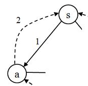
This applies only to the residual graph (so far). In this same maneuver, if we had decided to spend 2 units of flow from s to a, we have just described our adjustment to the residual graph. However the flow graph that we are building would also have to be modified; it would get an increase flow in edge (s, a) of 2 units. After all, our purpose of using 2 of the 3 units of flow from the residual graph was to produce 2 actual units of flow in our flow graph. I won't picture that here. Just remember that making any decision about using flow from the residual graph involves two parts:

1. adjusting the residual graph to reflect the used flow, and
2. adding this flow into the flow graph.

Section 11B.1.3 The Data Structure

Surprisingly, we can use our existing graph data structure organization with very little modification. You might think from the above discussion that we need to keep track of two separate graphs in two separate data structures and coordinate the action between them. Certainly, this is possible, but it is not necessary. Because the vertices are identical in both the residual graph and the flow graph, we can use the same vertex set for both graphs. In fact, if we use FHgraph as a guide for building FHflowGraph (our new class) we won't change the data - only the algorithms: we will replace the dijkstra machinery with maximum flow graph machinery.

So, where and how do we actually store the fact that there will be two graphs in this class, instead of one? In the vertex data structure. Remember that it is in that class that we represented the edges and costs, so all we have to do is keep track of two adjacency lists for each vertex. Instead of adjList, we will have resAdjList and flowAdjList. To visualize this, look at vertex a in the above initial flow graph and residual graph. We will store a as a single vertex but having two adjacency lists, resAdjList and flowAdjList. Here is a picture of this new vertex data structure:

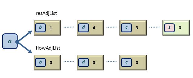
Compare this picture with the one above until you see it. (Question: why is there an extra vertex in the resAdjList?).

This is the only significant data structure change we have to make in order to do a nice maximum flow class. When we are chasing down paths or costs in the flow graph, we'll use the master vertex pointer set from our graph data structure, but we will look at each vertex's flowAdjList. If we want to do something with the residual graph, we will use the same vertex, but instead we will examine or adjust its resAdjList.

Section 11B.1.4 The Algorithm

We are now ready to describe the algorithm. The algorithm assumes that a start and end vertex are defined.

¹We discuss this step:

• in the residual graph add minCost to the reverse edges from start to end

The term reverse edge refers to the direction of that edge which is opposite to that of the path found in the current loop pass. It might be the actual reverse edge that we added when we initialized the residual graph - and for the first paths found it certainly will be. However, as the loop repeats, some paths found may use the reverse edges, which means in those paths, the reverse edge to which we will add the minCost in this step is actually the original direction of the input graph. This is a non-issue when implementing, but for understanding the algorithm we have to understand the meaning of "reverse edge" in this step. It is only "reverse" relative to the path just found.

²We must also remark on this step:

• in the flow graph add minCost to all edges from start to end along the path just found

Since the path found in the residual graph could use some reverse edges, there may not be a corresponding edge in the flow graph. That's fine; it means that we are changing our mind. We do this by subtracting the cost at that edge. In practice, we first look for the corresponding edge in the flow graph and if we find it we add the cost. If we don't find it we will certainly find the edge in the opposite direction and we will then subtract the cost from that.

³Finally, look at this step:

• find some path from start to end in the residual graph (the choice of path here determines the characteristics of the algorithm)

The only significant sub-algorithm that needs attention is the selection of a path from start to end. You can do this in many different ways. You can use what is known as a depth-first search to find any path that connects start to end, and return the first one you find. However, it would be nice to pick a path that has larger, rather than smaller, cost (flow) since that will often get us where we're going in fewer loop passes. One way to do this, and the easiest for us, is to simply cannibalize our dijkstra algorithm so that it has the following changes:

1. It uses start as its reference vertex.
2. It stops as soon as we pop end onto the partially processed vertices, for then we have found a path to end. It does not have to be the least flow, and in fact, it is probably better if it stops before finding the absolute minimum, since, after all, we are looking for maximum flow. However, it is not clear that finding either the minimum or maximum flow in this step helps our cause, and any path we find will work.

There are a million ways to choose the path, and a thousand variations of this one dijkstra-inspired approach. I am giving you one that requires the least amount of coding if you start with the graph template we already have.

The proof of termination and correctness of this algorithm are too technical to present here. However the coding and verification that it works are well within our means and it is part of your last program. I will guide you through that in your final assignment description.