Section 1 - quickSort

9A.1.1 Idea Behind quickSort

quickSort is currently the fastest sorting algorithm for general purpose use. Strangely, it is only O(N²) and this bound is tight (we can find an array that costs this much), but its average running time is NlogN. Furthermore, the constant time factors within this algorithm are much shorter than those in other algorithms, meaning that even though its running time may grow at the same rate as another algorithm, the actual elapsed time on most sized arrays is better than these other algorithms. We saw this effect with insertionSort, which was the same O(N²) as bubble sort, but beat the pants off it.

Also, quickSort is "in-place", meaning no extra memory need be copied to implement it.

The idea behind quickSort is simple.

1. Pick an element at random from the array. Call this the pivot.
2. Use the pivot to group the other elements into two groups: those < pivot (smaller subgroup) and those > pivot (larger subgroup). (Don't worry if duplicate elements == pivot might end up on both subgroups. This will not harm us.)
3. Recursively quickSort the two sub-groups (remember recursion works without explanation, on a smaller sized array or on the "lower level", always!)
4. Assemble the final array: smaller sorted subgroup, pivot, larger sorted subgroup. It is sorted.

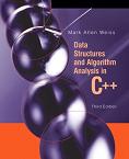
Here is a symbolic representation of this process:

quickSort's speed depends not only on fast inner loops but also on a good choice of pivot -- i.e., one that tends to break the array into two equal subgroups. If that is not accomplished, we end up with actual N² running times.

9A.1.2 Selecting the Random Pivot Element

The wisdom of hindsight allows us to select from among the best quickSort implementations, and we follow the text's version. The first step, getting a pivot, is oddly one of the most troublesome. Most arrays tend to come to us partly sorted, and even if they don't, once we start applying our algorithm recursively, it is easy to end up in some lower recursive level where we have, unwittingly (or wittingly?) given ourselves a sorted sub-array on which to work. With this in mind, we need a method of picking a pivot that doesn't result in lopsided subgroups when applied to a sorted array. A little thought (or pencil pushing) will convince you that using array[0], for example, as the pivot results in a nesting of recursion calls, each one of which is only one element smaller than the last. Summing these up gives the worst-case O(N²) performance. On the other hand, attempting to use a random number generator to choose the pivot can also lead to trouble as a call to rand() does take time, and that affects our algorithm's efficiency.

Median of Three

The time tested technique for getting a pivot is the median-of-three approach. Take the three values on the left, right and center of the array, and determine which one is the median (middle) value. We use that as a pivot. For example if array[] has 100 elements, and the values in the left, right and center are:

      array[0] = 932;
      array[99] = 37;
      array[50] = -10;

Therefore, we choose the median of 37 as the pivot. You could use more elements (five, seven, etc.) in hopes of the median being closer to the true median of the entire array - the ultimate choice -- but the more you use, the longer it takes to compute the pivot, while these extra elements don't seem to improve running times. So, three is the common choice.

9A.1.3 Approaching an Algorithm

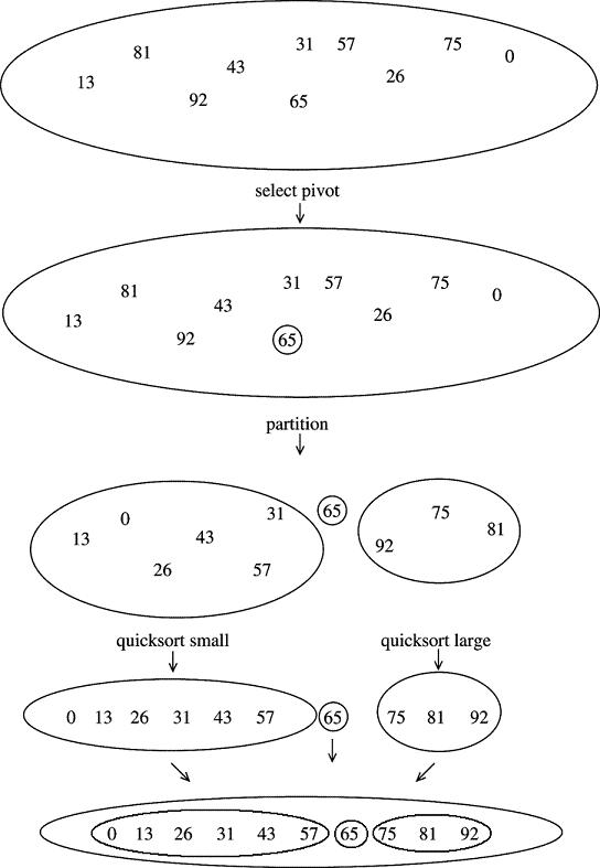
Let's make the above abstractions more concrete. Assume the input array is the following 15 numbers:

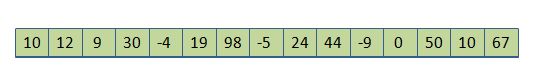
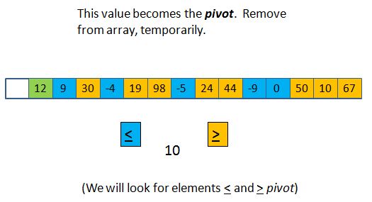
Median-of-three produces a 10 as the pivot:

Next, we will "remove" the pivot from the array (conceptually, probably not really), and then look at what is left. How do all the remaining 14 elements compare with the pivot? Some are larger, some are smaller:

Through a sequence of swaps, we will get the smaller subgroup on the left of the original array, and the larger subgroup on the right.

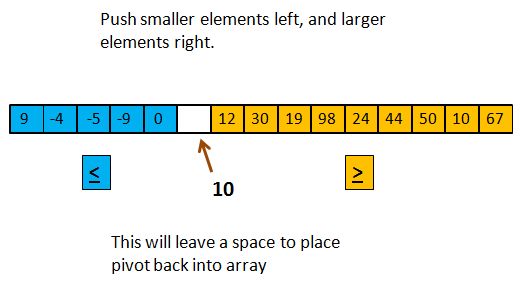
The elements in each sub-group are not necessarily sorted, but they do have the desired relationship with the pivot. They will also leave an unused location between the two - the position where the vacated pivot position has migrated. We can put 10 back into that position and it will be the final resting place for the pivot. Meanwhile, we are ready to call the quickSort algorithm recursively on the two smaller sub-arrays (the diagram below shows the picture before the recursive calls, so the sub-arrays are not seen to be sorted yet):

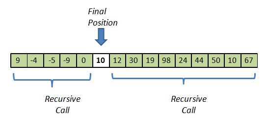
This completes the recursive step, and therefore the entire algorithm. I didn't describe, yet, the exact point at which the recursion ends. However, there is at least one obvious answer: if a sub-array size is 1, return.

9A.1.4 A Good End to Recursion

The algorithm described above is about ready to be coded. One difficulty is non-recursive "escape valve". Stopping at size 1 might be too late. For instance, how does the median-of-three work on 2 elements? It pays to stop the recursion before we get to 1, and it so happens that we should not even let ourselves get close.

quickSort is great for arrays that are not too small, but when you get down to 5 or so, the bookkeeping involved in median-of-three, combined with the recursive overhead, starts to have a negative cost-benefit.

So an elegant solution to all of this is to simply call insertionSort when the array size is 15 or below. This is exactly what we do.

(Tests show that if you break off recursion at different values from 100 down to 2, then times reach a minimum at about 25 and stay there until one gets to about 3 or 4 where times get longer. Any value between 5 and 25 seems to work the same, so I chose 15 for my coding. However, you cannot take my word for it, and you won't; this will be your assignment.)