Section 1 - Priority Queues and Binary Heaps

7A.1.1 Black Box Definition of Priority Queues

A priority queue is a data structure that has only two required operations and one requirement of its underlying data type:

• The underlying data type must have an ordering operation, usually realized by an overloaded < operator. This operation defines the priority of an object. We will proclaim the priority to be higher for lower ordering values, i.e., a has higher priority than b if a < b, by agreement.

The two required operations are:

1. insert(): there must be a means of inserting objects into the priority queue.
2. remove(): there must be a function that returns and deletes the smallest (or largest, depending on the requirement of the client) object in the priority queue. Since we are declaring high priority to mean a low ordering value, we will use remove() to remove the smallest key in all discussions and coding. This is our choice, and other development environments may define it opposite.

This is a very modest requirement for this ADT and we suspect that implementing it would be very simple.

In fact, we can certainly implement an inefficient priority queue immediately by wrapping a BST into a user-defined container and offering our users only the insert() and remove() operations which we would implement internally using the BST::insert() for insert() and a combination of BST::findMin() and BST::remove() for remove(). Or, we could "go Neanderthal" by using a vector and mapping insert() to push_back() and implement remove() using a short method that iterates through the vector finding and returning/deleting the minimum item in the vector. So, we have no shortage of unsophisticated and expensive ways to deliver something as externally simple, as a priority queue.

The challenge, of course, is to implement the priority queue efficiently.

Examples of priority queues are found within operating systems or programs that manage multiple tasks simultaneously. An operating system that has several processes which are active -- more than the number of processors on which to run them -- must store the processes on a priority queue and constantly find the highest priority processes to be executed, leaving the others in a wait state within the priority queue. There are other task-specific priority queues which pop into existence as well, such as those managing print tasks or instant messaging. In process control of machinery or in robotics there are various environmental factors that pose dangers or challenges to the equipment, and priority queues are needed to quickly pull off and dispose of those of highest priority.

You'll note that we don't really care so much about internal ordering in a priority queue. It is only being asked to give us the minimum. All the other objects can be jumbled in any order. So, while the < operator is important, we do not require that items be carefully sorted internally, which is one reason why a BST is overkill for a priority queue implementation.

This is the first time in several lessons that we find ourselves studying an ADT that has a direct implementation in the STL called the priority_queue. There were no hash tables, AVL trees, BSTs (or any trees at all, for that matter) in STL. The last data structure that we tackled which had an STL implementation was list, and before that, vector. Therefore, it behooves me to briefly mention the terminology for STL::priority_queue.

1. insert(): This is implemented using a method called push() in STL priority_queue.
2. remove(): This is handled by a one-two punch typical of STL methods: pop(), which removes the minimum without returning it, and top(), which returns it without removing it.

This tells us that priority queues don't typically have the simple two methods insert() and remove(). For STL, when we want to perform a remove() we will first call top(), and follow it with a call to pop().

In another twist, STL::priority_queue is a special kind of class template called an adapter. Yes, it is a template, and you can even use it just like a list or vector, specifying only the underlying data type in angled brackets. However, the priority_queue actually implements itself using some other container whose choice is up to you, the client. If you don't specify anything special, it will use a vector. However, you can tell STL::priority_queue to use a dequeue, instead. I won't bother with the syntactic details here, as you can look them up in the STL reference online.

7A.1.2 Binary Heaps

Priority queues are almost always implemented using a data structure which is perfectly suited for them: the binary heap. We will see that binary heaps have other applications as well, one such being a fast, O(NlogN), sort called the heap sort. Remembering that we are considering minimum to be high priority, we will be dealing with what are sometimes called min heaps, in contrast to max heaps, which have the high priority items possessing large "keys".

The binary (min) heap has the following properties:

Structure Properties

• The tree is a binary tree.
• The tree is complete.

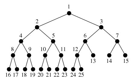
A tree is complete if the only nodes missing (i.e., preventing it from being a perfect tree) are in the bottom level, and the missing nodes are all on the right portion of that bottom level. Another way to say this is that we can read off the nodes of the tree from top to bottom, left to right, and we will be reading off totally filled levels until we get to the final, bottom, level where we will have every node occupied up to a point, at which time, there are no more nodes. Here is a nice picture that gives the completeness idea:

Heap-Order Property

• The root of the tree (or any subtree), is the smallest node in the tree ( or subtree).

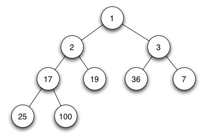
The ordering condition makes no claim about the in-order traversal being sorted, and in fact, it cannot be a BST because this ordering property conflicts with the BST ordering property. The above tree is easily verified to be a binary (min) heap as are the following

We can see part of the utility of a binary heap in implementing priority queues -- when we want to do a remove() or any version thereof, we know where to go -- the root has the node we want. It is as fast an operation, O(1), as we could hope for. That explains the purpose of the heap-order property. The use of the completeness structure property is not as evident, but here are a few clues:

• It gives a very balanced condition, which leads to fast search times.
• It is possible to accomplish completeness with the weak ordering condition such as this. If this were a BST, the completeness requirement would make for an impossible data structure. So, the heap-order property allows that we can at least contemplate completeness.
• It turns out that completeness makes for a tree implementation which is extremely fast and elegant. In particular, we will be able to use a simple fixed-size array to hold our binary heap ("fixed size", that is, until and unless we need to increase it due to the underlying array becoming full, a relatively common situation that we fix by doubling the size, as usual.

7A.1.3 Vector Implementation of Binary Heaps

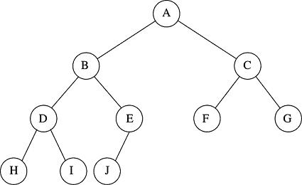
Take the last diagram as an example. We will show how an array or vector can hold this data to our advantage. Since we know every level is completely full, we can simply store data into the vector by reading through the heap left-to-right, top-to-bottom. As we come to each node, we store it in the vector. The only condition is that we start filling the array at element 1, not element 0, for reasons that will become clear. Here is the internal representation of the above binary heap:

The root value, A, is stored in location 1. Its two children, B and C, are stored in locations 2 and 3. B's two children, D and E are stored in locations 4 and 5. C's two children are stored in locations 6 and 7. And so on. Here is the formula for this situation:

Bin Heap Array Rule

Any element at position k has a parent at position k/2 (integer arithmetic). If the element at position k has a left child, it can be found at position 2k. If it has a right child, that one can be found at position 2k+1.

Loosely speaking, you get to a node's parent by dividing by two. You get to its children by multiplying by 2. You can imagine how powerful and elegant this situation is when it comes to coding algorithms.