Section 1 - Open Addressing

6B.1.1 Linear Probing

Hash tables are often used when access is time-critical or space for data and program is limited. In such situations, separate chaining is not desirable because of the overhead involved in the list data structure for each bucket. A solution which involves only an array (or vector), and no lists, is called open addressing. Here, it is possible to place an element into an array location that is not, precisely, the one selected by the hash function. If a collision occurs, we probe for alternative locations and use those alternatives as they arise. For this reason, hash tables which use open addressing are called probing hash tables.

Consider insertion. The idea is straightforward, especially if we implement the simplest form of probing called linear probing. We are using arrays, now, and nothing else. So if there is a collision we have no alternative other than to search elsewhere in the table for a vacant location. The obvious idea is the next location in the array. So if

index = hash(key)

takes us to an array element, mArray[index] which has an active element in it, we try the next location mArray[index + 1]. If that is occupied, we try mArray[index + 2], and so on until we find a vacancy. For removal and containment, the algorithm is similar. If we use a simple key % 13 hash function for a hash table of size 13, then start inserting nodes 18, 41, 22, 44, 59, 32, 31 and 73, we would get the following:

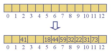
Frequent collisions (starting with the fourth insertion) cause a cluster of contiguous occupied cells. This clustering is caused not only by hash function collisions, but by a secondary effect: the hashing function sometimes maps a new key into the middle of an existing cluster -- a position that was not actually hashed before. It results, nevertheless, in a collision, and the new element will linearly probe from there to the next free location, causing that cluster to grow even larger. For this reason, linear probing, while a simple conceptual solution, is rarely used without some modification.

One modification is to provide a secondary hash function, and this is called double hashing. I will not consider double hashing in these lectures, but you can read about them in your reference. Instead, I will talk about a different solution to the clustering problem called quadratic probing. It is very fast and effective, and is used frequently. We'll do this fast and furious technique in an up-coming section in a few moments. Rest up.

6B.1.2 The HashEntry Data Type and Lazy Deletion

Before digging into quadratic probing, we can see certain issues that will come up with any open addressing scheme like linear probing. First, the labeling problem. How do we know if an element in our array is occupied? We can't tell by looking at the data. We must therefore add a member to the element data type which I will call the element state or just state. It can be ACTIVE or EMPTY meaning occupied or available, respectively. To do this, we really need to create a new data type to act as the underlying type for the vector. vector<Object> no longer works. We create a new type, called HashEntry:

template <class Object>
class FHhashQP<Object>::HashEntry
{
public:
   Object data;
   ElementState state;
   HashEntry( const Object & d = Object(), ElementState st = EMPTY )
      : data(d), state(st)
   { }
}

This code comes from a template where we are defining an outer class FHhashQP, which is why we see that in the notation. (It shows the notation for nesting a class type, HashEntry, in a template, FHhashQP, and this particular example shows the external definition of the nested class.) However, the important thing is the idea that we have embedded the data into a slightly larger envelope that includes a state member.

The second problem is the deletion problem. We cannot simply mark an element as EMPTY if we want to delete it. If we did, it would produce a gap in the cluster, cutting off all the elements to its right from being "found". A contains(), insert() or remove() operation will start with the hash location, and move right until it finds an EMPTY location, then assume that it has exhausted the probed locations, reporting that the element was not in the table. For example, if we remove 59 from the above table we end up with a gap:

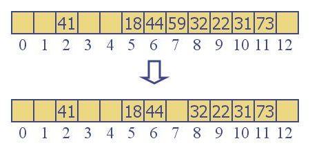
Now, what happens if we try to call insert(32), contains(32) or remove(32)? 32 hashes to 32 % 13 = 6. From there it probes until a vacancy is found in mArray[7] (the 59 may still be in that location, but it has been marked EMPTY). Regardless of which of the three methods we are trying to invoke, the wrong thing will now happen. The 32 was not detected but should have been. For this reason, we see that ACTIVE and EMPTY do not constitute a sufficient set of flags for our state variable. We'll need a DELETED value as well, indicating that this location has no data in it, but it must be considered occupied for probing purposes. When we see ACTIVE or DELETED, we have to continue probing.

This idea is something we have discussed in trees -- it is called lazy deletion. In this lesson, we are going to implement lazy deletion. It tends to be lazier when we are using lists rather than open addressing, but the term still applies - we are refusing to truly delete the data, and instead marking it as DELETED.

Notice that we cannot really use a DELETED location (at least not immediately) to store a new element because the first time we encounter it in an insert() invocation, we are not sure that the element we want to insert is not already in the table. We have to keep probing. By the time we are done probing, we are at a truly vacant location, and it is there that we usually decide to store the new data.

This comes up in all probing (including quadratic probing) as well as double hashing.

This is not to say that there is not a solution without the DELETED tag. One can fill the gap during deletion. I'll leave that as a topic of discussion or perhaps a homework assignment.