Section 1 - Hashing Fundamentals

6A.1.1 Hash Tables and Hashing Functions

We seek an alternative ADT that has fast access properties. The member of the underlying data structure which determines where we store our element will be, as usual, informally called the search key, or key. Our goal with this new structure is:

1. O(1) access time for every element in the ADT
2. Support for search keys which are not integers (e.g., strings), or, if they are integers, have widely divergent values (3, 190, 10 billion, -89433, etc.)
3. No ordering built-into the underlying data type
4. == and != operations defined for the underlying data type
5. Infrequent re-structuring of the ADT

None of our prior data structures, except perhaps the array, will work. Since we want O(1) access times, trees and lists won't do. What about arrays or vectors? If the search keys are not integers, they won't work. If they are integers, the divergent nature of the ints, as described in requirement 2, rules them out. We can't easily allocate arrays or vectors whose index values are on the order of billions, especially if we don't expect to make use of most of those array locations.

There are two very common examples of kind of data. First, there is the phone book data base. There we have name/number pairs, and the search key is a string, the name. We will use the name to store and retrieve the pairs. Secondly, we look at an employee or government data base, in which names, addresses, incomes and social security numbers are the data. This time, the unique key is the social security number (ss#).

Let's consider the latter example first. We want to be able to take a ss# and use it to find, very quickly, the record. In a theoretical world, we would use the ss# as an index to an array. However, that would require over a billion array elements, and we would be using only a fraction of them -- maybe a few hundred, or thousand -- to actually store data. We want something like an array, but without the memory requirement or space wasting side-effect.

The solution is to use an array whose size is guided by the number of items we expect to store, not the ss# range. This will be our table or hash table. Next we use the numeric ss# key as an input to a function, called a hashing function or hash function, that will then produce a smaller number we can use as an array index. We call the function hash(), and the return value of the function:

index = hash(ss#)

will be smaller than the ss# and be something that we can use to access our table. Let's say, for example, that we have a company with fewer than 1000 employees, so an array of size 10,000 would be fine to store all their data, including an allowance for future growth. In that case hash() will return a value between 0 and 9999, and this value will be the place where we store our employee record. Here's a picture:

In the above picture, the hash function, hash(), would turn the ss# 025610001 into the index 1, i.e., hash(025610001) = 1. Similarly, hash(200759998) = 9998. The main requirement of a hash function is that it reduce the key into a relatively small int that will lie within range of our target array (the table). Although I haven't given you the definition of hash() in the above example, I am confident that you can guess what it is. Take a look at the picture, and think. This is not the only possible hash function for this application. There are infinitely many choices, and one of the tasks of an ADT programmer is to select or devise a good one.

(Side Note: I fully expect and encourage anyone who has the above social security numbers to sue Foothill College.)

The array elements in the table are sometimes called "buckets" because we will see that they sometimes hold more than one record -- they hold a bucket of records.

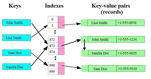
Here is the hashing function concept applied to the phone book example, where we use the name key as input to a -- for now -- unrevealed hashing function:

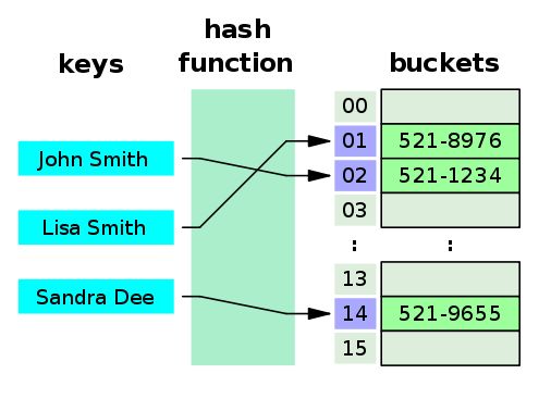
In this case, we are only storing the phone numbers because we really don't need the names. In this application we just want to use the name to find the numbers. Plug the name into the hash function, get the number, and we can report back to the client. Or, use the name to compute the place in the table where we want to store a new phone number.

6A.1.2 Collisions

By now, some of you are not buying what I'm selling. For example, in the ss# example, you probably guessed the hash function, so know that we'll have a problem if I attempt to store an employee whose ss# is 981100004 into the above hash table. Look:

The problem is, of course, that the hash function mapped two different ss#s to the same bucket. It is an occupational hazard of hash tables. We have to build-in the accommodation of this eventuality. In the phone-book example, if we use a slightly different hash function than the one indicated in the first diagram, and attempt to store four records the same thing can happen:

When two keys are mapped to the same bucket, or table entry, we say a collision has occurred.

This motivates us to make our table more than a simple array of records of the underlying data type. It must somehow allow us to store more than one record in each table location. There are a number of ways to do that, the most direct of which is suggested by the last diagram. If you look at how the two colliding phone records are stored in bucket 873, you'll notice that a linked-list structure is pictured. That's exactly how we implement the first hash table flavor, Separate Chaining Hash Tables.

In separate chaining, our hash table is an array of LinkedLists or more often, a ArrayList of LinkedLists. (I will call LinkedLists just lists in much of this discussion.) If we want to find an element in the hash table, we compute its key, which immediately sends us, in constant time, to one of the buckets. From there, we have to traverse a, hopefully short, list of elements, all of which collided when they were originally placed into the table. If you can imagine that we will design the data structure in such a way that only one or sometimes two -- and rarely three or more -- elements are in each bucket list (!) then you see that the list traversal is practically insignificant from a timing standpoint.

That's the big picture in all hash tables.

1. Define a vector of lists or something similar to hold the items.
2. Define a hashing function that turns keys into an array locations -- a bucket.
3. Traverse that particular list until you find the record in question (this is where we'll use the == and != operations of our underlying data types).

6A.1.3 Hash Functions

We first have to deal with the choice of hash functions. The goal of a hash function is to produce an int which maps to all index locations with equal probability. This will result in the fewest collisions and buckets with approximately equal numbers of members. We will spend a whole page discussing this matter.

6A.1.4 Table Expansion and Load Factor (λ)

Our goal is to have an O(1) search time. However, we can't really guarantee this. If we are very bad at writing hash functions -- or very unlucky with our data -- all of our keys will be mapped into very few buckets. This means we'll have a few long lists and lots of empty lists. Of course we really won't be bad at writing hash functions because we all will have completed CS 2C from Foothill College. However, we cannot control the incoming keys. In order to ease the population explosion in our buckets, we occasionally double the size of the hash table, much as we have done with vector implementations.

There are two innate numbers, and one computed number, that are very important in determining our search time. The two innate numbers are:

• tableSize - the number of elements in the ArrayList or array. This number is usually a prime, as you'll see.
• size - the number of elements in the hash table to date.

If, for example, tableSize is 101 and size is 200, then, if we had a good hash function, we would expect the typical bucket to contain two elements. This implies that our search time would be the constant time to compute the hash function plus 1.5 × [the time to jump to the next element in our bucket list]. I say 1.5 because that is the average number of jumps in a list of two elements. (Well, not quite, because every time we search for something not in the list, we always traverse both elements and return false, so this causes the analysis to tip in favor two iterator jumps rather than one, but 1.5 is close enough.) If we had 600 elements stored in the same table, we would have, on average 600/101 or six elements per list, making our average search time through the list three jumps × [the constant time for a jump]. (We always add the hash computation to every search, so I'm going to stop mentioning that).

With this preparation, we define the load factor, lambda (λ) to be the changing number size / tableSize:

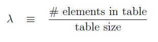
With this new vocabulary item, we can say that our search time is going to be O(λ/2) which is, of course O(λ). We will now include a member, mMaxLambda, to be part of our data structure. We will not allow λ to get larger than mMaxLambda. For instance, if we desire an average of zero collisions, we will set mMaxLambda to 1. when λ gets larger than this, we have about 1 item per bucket. It is then time to increase the table size, and we do that by resizing our hash table, or rehashing.

Setting mMaxLambda to 1 or 2, or even 3, is fine for separate chaining hash tables, because, really, jumping once or twice is not normally a big deal. Still, if we are doing hypercritical development (programming a compiler, doing real-time simulation, etc.) we can and will set mMaxLambda to 1 or even .75 or .5, thus making sure that search times are short. Don't forget, though, that when you set a lower mMaxLambda , you are going to cause a rehash maneuver (doubling the size of, and rebuilding, the hash table) sooner and more frequently. Rehashing is done during insert() operations, so a smaller mMaxLambda will cause an occasional slow insert().

For separate chaining hash tables, mMaxLambda = 1 is fine. For probing hash tables (coming soon to a theater near you), mMaxLambda must be, at most, 0.5, and to be on the safe side, literally smaller, such as .49, to avoid computer round off error so that we never go above 0.5.