Section 5 - Splay Pictures

5B.5.1 Preliminary Remarks on Comparative Terminology

My terminology below is slightly different than most of the literature.

Only Two Conditions

My discussion investigates two, and only two, conditions:

Zig-Zig: when the value for which you are splaying falls in the same direction twice in a row off the root: right-right or left-left.
Zig-Zag: when the value for which you are splaying falls first right then left (or vice versa).

Note that these are conditions, not operations. Each condition has its corresponding usual operation which is performed when the condition is detected. Thus, when we detect a zig-zig condition we do the usual zig-zig operation, and when we detect the zig-zag condition we apply the usual zig-zag operation.

It is possible, however, that we hit a null or the value for which we are splaying while processing one of these two conditions. If so, we may have to veer from the usual operation slightly. Some authors like to give different names to these alternate operations (single zig or simplified zig-zag), but I prefer the simplicity of organizing our logic into two simple conditions and their corresponding usual operations. Therefore, you will see only two cases, below, and the operational responses to those. Try not to worry about any special sub-cases, since they are handled in the algorithm itself, without assigning labels to those cases.

My Terms vs. The Book's

Zig-Zag: If you have read other authors or studied the text first, then be aware that what I call a zig-zag operation is what is often called elsewhere a simplified zig-zag. I do not even discuss or use the full zig-zag operation of some other authors. Remember, the condition is the same: zig-zag. The difference is what one does when one detects that condition, and in my development, I always take the simple route.

Zig-Zig: My zig-zig operation is equivalent to the book's. The book goes on to differentiate a single zig, but I do not. That situation is handled naturally with an if statement in the algorithm as part of processing the zig-zig condition. I don't give it a special case.

5B.5.2 Zig-Zig

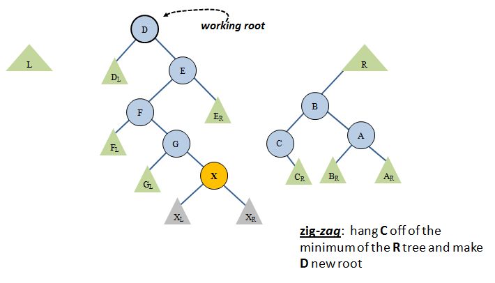
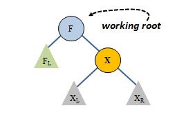
We now explain exactly how nodes are moved from the main tree to the L and R trees. Let's say we are at some intermediate phase of our splaying where we have three trees, L, R and main. Let's say that we are splaying for X (I'm switching to capitals because they look better in the pictures) and X is, indeed, in the main tree. Here is a picture of the three trees, including the names of some of the nodes on the path to X:

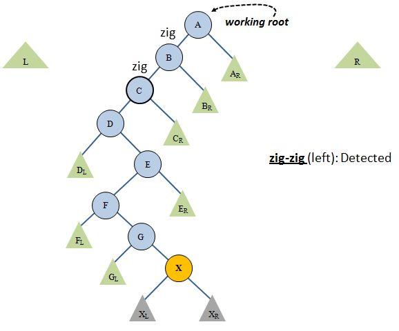
A is the working root. By comparing X to A, then B, we find that we need to move left twice on the path to X (X is strictly < A and X is also strictly < A's child, B). This is called a zig-zig operation, because we move in the same direction twice (left-left or right-right). Assume, as the picture suggests, we are doing a left zig-zig. When we detect a zig-zig our immediate goal is to move the grandchild (C) to the working root of the main tree. To make this happen we will:

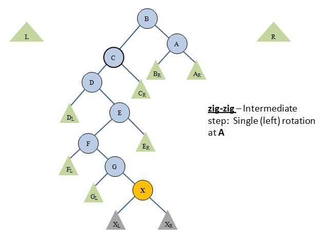
Do a single rotation (left, in this case) at the working root, A, which will bring B to the working root position. This is the exact same single rotation you learned in AVL trees. Hurray - no new code to write.
Prune B (the new working root) from the main tree and "graft" it onto R. When you do this, one of B's subtrees (the one that contains A -- the old working root) will go with it to its new home, R. Specifically, it will be placed to the left of R's minimum node, since B and all that hangs from its right side must be less than everything already placed into R. (This last assertion requires a short proof which I will leave off the page. You can take my word for it, or spend some time figuring out why it must be true.)

Here is a picture of these two operations, first the rotation:

Next, the transfer to the R tree:

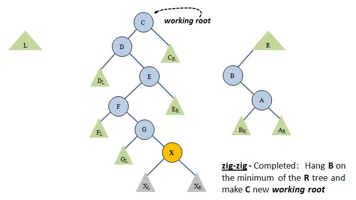
Now we have shortened the main tree by two levels and added some things to R. (Of course, if the zig-zig had tilted right, we would be doing the mirror image, adding stuff to L).

5B.5.3 The Zig-Zag

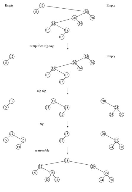
The other possibility is that we do not have a zig-zig condition as we move from the root down toward X: We have a zig-zag, wherein we move left-then-right, or right-then-left. In fact, that's what happens at the very next pass of our loop in the above diagram. Look:

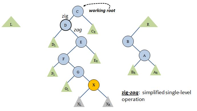
In this case, you deal only with the immediate child of the working root (D, above), lifting it to the root position, and moving the old working root, C, to the appropriate L or R tree. In this case, since C > X, C will be placed on the R tree. There is no rotation in this case. It is actually nothing more than the second of the two steps in the zig-zig case, so it is shorter:

Again, the place where we put C, the old working root, is at the left child of the minimum of R.

Look at what's in the main tree and you'll see another zig-zag, and after that yet another zig-zag. After both of those operations you have:

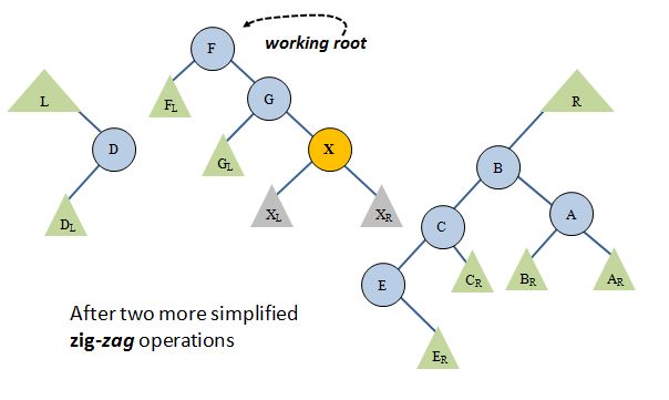
Make sure you get the same answer if you do the two zig-zag operations.

We're almost done. We finally have a zig-zig operation (right-right). Repeat the logic of the zig-zig we saw before: do a single right rotation at F followed by moving G (the new working root after the rotation) onto L; specifically, hang it off the right child of L's maximum node:

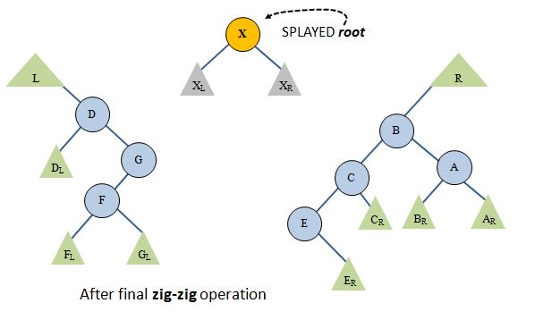
Aha. We found X. We are done splaying. All that's left is to assemble the three trees:

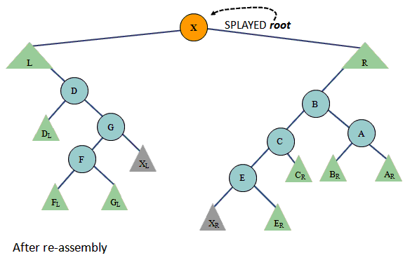
Look carefully at where X's left and right subtrees landed. During the final assembly they were moved to the "bottom" of L and R, respectively. After that happened, we attached L and R to X as children. As I indicated, if you were to go through a rigorous recursive analysis of what just happened, whenever we put something, like X_L into the L, we always place it as a right child of L's maximum. Likewise, anything added to R, like X_R, will always go below and to the left of R's minimum. You don't need to fully "see" this, but you do have to implement it. It is very easy, because you will naturally have variables called leftTreeMax and rightTreeMin which always point to the exact nodes where you will be hanging new fruit trimmed from the main tree.

5B.5.4 The Simple Zig

You might wonder why I did not mention the single zig move. Other authors include this. First of all, what is the simple zig? It is the case where our target node, X, is a direct child of the working root:

But if we test for zig-zig first, as we always will do, then when a zig-zig is not detected (we do not move left-left or right-right) then this case will appear identical to the zig-zag case. That's because we will test

if (X < root) && (X < root's left child)

for a left zig-zig, and

if (X > root) && (X > root's right child)

for a right zig-zig. If X happened to be the working root's child these conditions will test false exactly as they would in the full zig-zag situation.

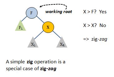
The result is that we apply zig-zag rules, lifting X to the root. Thus, if X is in the tree, it will end up at the working root, either by a final zig-zig operation, as we saw previously, or a final zig-zag operation as we see here. In summary, the simple zig is subsumed by the zig-zag case.

5B.5.5 What If X is Not In the Tree (We Hit a null)?

The above operations assume that we can move down from the root twice on the way to X without hitting a null. That's fine. If we do hit a null, we will break out of the splay loop and not attempt the pruning portion of the operation. This will be expressed in the algorithm on the next page.

We complete the description of the top-down splay by considering the situation where we don't find X. The only way this can happen is if we attempt to move left or right from the working root and find a null. If this happens we stop splaying and allow the working root, say Z, to be the final splayed root. We re-assemble the tree exactly as we would if we had found X, the only difference being that rather than X appearing as the final splayed root, Z is. This is advantageous if we are trying to insert X into the tree. If we splay first, and find that X is not at the root, the splayed tree will have left the tree in a perfect situation for inserting X. You'll see this in the insert algorithm.

Here is an example of top-down splaying when X is not in the tree. X = 19 is the target of the splay. Bear in mind that this is the author's terminology. What the author calls a simplified zig-zag is my one-and-only zig-zag. Also, the author's final single zig is my normal zig-zig condition. The difference is that my algorithm will terminate before the pruning portion of the zig-zig. However, after the reassemble step, both algorithms produce the same final tree.

5B.5.6 Inserting into the Splayed Tree

Consider insert() now. This method will first call splay() passing the target, 19, to be inserted. If 19 is not found in the splay, as shown above (just look at the root and if it isn't 19, 19 must not have been in the tree!) then it will be very easy to insert now. We will do that and simultaneously make the newly added 19 the root of the tree by:

Create a new node and put 19 in it as data. This is going to be the newRoot of the tree.
Because the splayed root, 18, is < 19, place 18 as newRoot's left child.
Place 18's right child as the newRoot's right child.

Since splay() will guarantee that everything in the left subtree of the splayed result is always strictly < the target data, and everything in the right subtree is strictly > the target data, the above three step procedure works.