Section 4 - Top Down Splaying

5B.4.1 Splay Trees

A Splay Tree adds an additional requirement to balanced trees: the most recently inserted or accessed node in the tree is repositioned at the root of the tree. This implies that any subsequent accesses of that node are very fast (O(1)). The idea is that once an item is accessed, it will likely be accessed again, very shortly afterwards, by the client. This assumption is true for many real operating system applications. One spends a little more time during the first access to that node in getting it to the root, but this time is amortized over the next several accesses which find() that node instantly, due to its being at the root of the tree. Even if other nodes are accessed shortly after, this node stays near the top, at least for a while, so it will be readily available in the short-term. It won't be until after many accesses of other nodes, that it falls back down toward the bottom of the tree. As in all BST species, there is a cost benefit. If nodes are accessed truly randomly, with no relationship between one access and the next, then Splay trees become expensive and slow.

5B.4.2 Splaying

The idea of splaying involves starting with a tree, T, and an object, x, that may, or may not, be in the tree. We will perform a splay operation on T, relative to x that will restructure T so that x will be at the root T after the operation (if x was in T). If x was not in T, then the splaying will have left T in a perfect state for the pending insertion of x: We will be able to insert x directly at the root of the recently splayed tree by adjusting a few links near the splayed tree's root.

This is called "splaying x in tree T", or since we usually know what tree we're talking about, just "splaying x".

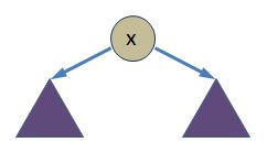
If x is in the tree, after splaying the tree will have moved x into the root position:

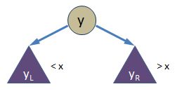
If x is not in the tree, after splaying the tree will be organized into a root (y) and two sub-trees; one is smaller than x and one is larger than x:

Splaying is not something that a client can or should call. It is a private matter that tree methods will invoke to assist with the usual operations like contains(), insert(), remove(). It is those public methods that will call the splay() function. Done correctly, splaying has two benefits:

1. It makes future access to the splayed objects fast.
2. It tends to bring items near the splayed object (and on its original path) closer to the new splayed root.

Thus, splaying tends to reduce the height of the tree. However, it only "tends" to do this, as you will see. It can make trees deeper if you get an unlucky combination of accesses.

The big result about splaying, which we won't even pretend to prove, is that the time complexity of M accesses of a tree that uses splaying is MlogN . This means that the average access is logN , which is what we want. We're looking for a way to bring recently-accessed data near the root of the tree without sacrificing the logN search times we've enjoyed with our AVL trees.

5B.4.3 Top Down Splaying

There are two types of splaying: Bottom-up recursive splaying and Top-down non-recursive (iterative) splaying. Bottom-up splaying is usually taught first because it is easier to understand, then ignored because top-down splaying is faster and easier to program. Yes, you read right: top-down splaying, while harder to understand, is easier to program. This week, I'm asking you to program, but not necessarily understand, top-down splaying. You need to know the algorithm, but not be required to fully comprehend why it works. You'll get the idea. I've got a few pictures in my pocket for you.

Going into this, remember what I said about the splay() function. We will write it as a stand-alone algorithm to be put in the private section of our splay tree class, but only invoke it during the definition of the other public functions. So your first step is get a feel for how it works so you can write a splay() function. Then, you'll be able to use it to implement insertion, removal, etc. And it will make those functions very easy to write.

The idea of top-down splaying is as follows:

1. It is an iterative (loop) process that always has three trees
   • The main tree that you are searching (which you expect contains x)
   • A left tree, L, which contains nodes less than x that you have already examined and can be safely moved "out of the way" of the main tree, and
   • A right tree, R, which contains nodes greater than x that you have already examined and can be safely moved "out of the way" of the main tree
2. Initially the main tree is the entire tree, T, that you are searching and L and R are empty trees.
3. As the splay progresses, you will be moving left and right down the path towards x, much like we have done in the past in such algorithms As you do, you will be removing nodes you encounter from the main tree and placing them into either L or R, depending on whether they are less than or greater than x. Thus, the main tree will get smaller, and the L and R trees will grow.
4. If you find x (or hit a null), you are done with the splay. You can then re-assemble the three trees by adjusting a few links and return.

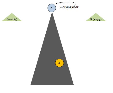
Here is a sequence of pictures that symbolize the initial, mid-process and final stages of splaying. First we begin with two empty trees L and R, and our original tree. Let's say the root of the main tree is initially A. This will be our working root. As the algorithm advances, these working roots will be tossed aside into either L or R and new working roots will take their place (until we hit x, at which time, we're done):

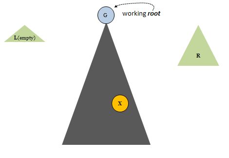
You can see x deep down in the main tree. We're moving toward it, getting closer each loop pass. After a few loop iterations A is replaced by other working roots. The main tree shrinks and the L and R trees grow, Here is an iteration on the journey which brings a node, G, to the root:

and later, P becomes the working root of the ever shrinking main tree:

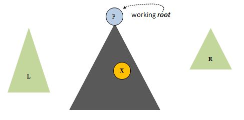
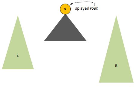
One day, if we're lucky, we find x at the working root. We are done with our splay process (L and R will not necessarily be the same size):

That's fine, but we have ripped apart our tree and now have three where we were given only one. No problem. Since all the nodes in L are smaller than x, and all the nodes in R are greater than x, we can hang L and R directly off of x as left and right children. When doing that we would lose the two trees below x (not distinguished from each other in the above diagram, but both part of the dark gray region below x). So before overwriting x's lftChild and rtChild links we will place those two sub-trees at the periphery of L and R, symbolically as follows:

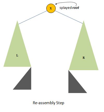
This is called "reassembling the splayed tree".