Section 4 - Analysis and Discussion of BST

4B.4.1 Big-Oh Estimates

We can do a rigorous analysis of binary search trees, but a little common-sense consideration will give us some useful insight. Look at this search tree - it has 11 nodes and height 3:

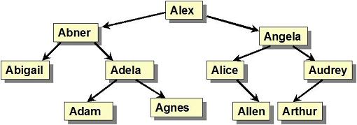
Recall that height is the path length from the node to the deepest leaf (from that node). So for a tree with height 3, we are certain to do no more than 4 comparisons for any search operation. We could even add more nodes and keep the height of the tree unchanged. As you can see, if the tree has N nodes we can, if we are lucky, have a height that is approximately, logN. Thus, we expect our search times to be O(logN).

There's another way to anticipate this same estimate. Remember this?

In a typical tree search, every time we move left or right down the tree, recursively, we have made a choice to forsake about half the collection, which means we are cutting the search space roughly in half each comparison. This satisfies the rule about logN search times.

But is O(logN) what we really get?

4B.4.2 Analysis When Height = M

Throughout this discussion, we take N to be the number of nodes in the BST. Let's not make any assumptions about the height of the tree yet. We'll say it is some value, M, but we don't know if M is large (close to N-1) or small (close to logN). Whatever M is, we can easily see that both the search and insert operations are O(M+1) = O(M), since we will never do more than M+1 comparisons, but in the worst case, we may have to go all the way to a deep leaf, suffering all M+1 comparisons This tells us that both search (and insert), which are basically the same algorithm, are O(M).

A remove is a little more complicated because in the worst case (i.e., two non-NULL children hanging off the node to be deleted) we recurse.

Simplistically, this forces us to recursively find a node to be removed (say found at height k) and, when found, call findMin() from there (cost = k) followed, in turn, by another recursive call starting at height k-1. Considering this description without looking at the details, we would conclude some hypothetical recursive call that employed findMin() prior to the next recursive call would take roughly

steps. (In that analysis, I assumed the each recursive call only brought us one step lower in the tree.) That sum is O(M²), i.e., quadratic on the height M.

However, in our particular remove(), if you follow the logic in the algorithm, you'll see that we really only have to search down from the root to the deepest node at most twice, adding both the recursive search steps and the findMin() steps. It turns out that all these comparisons, added together, count for, at most, 2M comparisons. So a removal is O(2M) = O(M). It's longer than search and insert, but it is still O(M).

Balanced Trees

In the best case, we are dealing with a symmetric tree, one that looks like this:

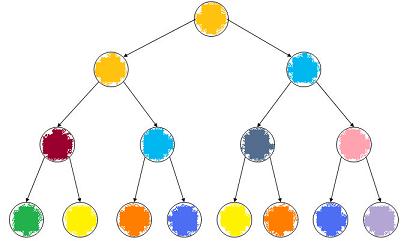
This is called a full tree or perfect tree: all nodes at depth K have the same height (which happens to be M' - K - 1, where M' is described in the next sentence). Full trees always have N = 2^M' - 1 nodes for some M'.

As you can verify, the height of a full tree is M = M' - 1 = log₂(N+1) - 1, which we'll just call logN, since the +1 and -1 have no effect on time complexity.

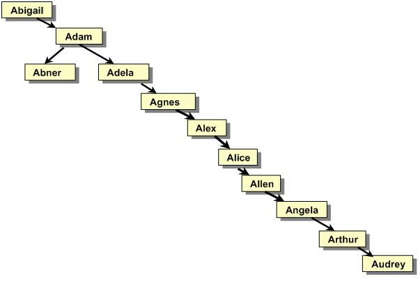
Unbalanced Trees

The opposite happens when every node has only one child. It doesn't have to be always the left or right child: all trees with exclusively single children nodes are the same height, namely M = N-1:

Even trees that are not totally unbalanced can be closer to height N-1 than they are to height logN:

In summary, if we have a BST of height M, actual search, insert and remove times are Θ(M), regardless of what N is. (with remove taking longer, in absolute terms than the other two). You should easily be able to convince yourself that M is always between logN and N-1. So, if we have a fixed tree that never changes, we have an answer, and that answer is good for balanced trees, Θ(logN), and not-so-good for unbalanced trees, Θ(N).

4B.4.3 Average Case

We now know how long an operation will take for a tree of height M, but we don't know what M, on average, is. We can compute it, and it is done in many places, including the text. Fix N, the number of nodes, then count all possible tree structures with exactly N nodes. Let's say there are S different ways to present the N items for insertion, that is, there are S ways to build a tree of N object starting from scratch and using insert(). Each distinct steam of data, which is represented in one of the S input patters, results is some tree. Call the kth tree, Tree_k. Tree_k has a certain height, call it height(Tree_k). To get the average height, add up all these heights and divide by S:

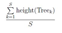
(S, by the way, is easily seen to be N!.) I'm not going to try to do the computation, but this is the direct way to compute the average height of a tree with N nodes. The result will be of the form KlogN, where K is a constant, so this makes the height of the tree O(logN), in fact, Θ(logN). This tells us that a tree generated randomly (no input/insert sequence is any more probable than any other sequence) results in Θ(logN) average running times for insert, search and remove.

The problems with this are:

1. We may not get our data randomly - it may come to us semi-sorted, and it often does (our Project Gutenberg data being a good example).
2. Once the tree is built, our remove algorithm tends to always lift the right subtrees up one level, causing the tree to be imbalanced -- weighted to the left.

There are work-arounds for each problem.

1. If we are taking-in a lot of data once, we can shuffle the data first, making sure it is random, before generating the tree.
2. In our remove(), instead of always picking the min of the right subtree, we pick the max of the left subtree half the time.

You have to do scenario testing in your application to know whether your trees are balanced enough to exhibit Θ(logN) running times. If they are, then you are fine. If not, you'll have to change from a simple binary search tree to an AVL, Splay or Red-Black tree structure, two of which we will cover next week.

4B.4.4 Trees vs. Binary Search

You have burrowed far enough into this course to be able to have an intelligent discussion about the relative merits of a BST and a simple binary search algorithm on an array. This is a conversation I have been wanting to have with you since the first day of class, and am thrilled to say that we are finally ready to have it. Have a seat.

We expended a lot of energy and gave birth to a few brain cells, all toward the goal of building a binary search tree. If you are absorbing the material well and reviewing past modules as you should (ahem...), the question presents itself - what have we gained? We already had a Θ(logN) search algorithm, so why do we need a new one?

True, our prior lesson's binary array/vector search is great and fast and wonderful, but it requires that the data be sorted before the search is begun. If we build the array once and never touch it again, that's fine, but we cannot insert, or even remove data without doing some heavy lifting on the array or vector to keep it sorted and free of holes (i.e., vacant locations). This heavy lifting takes the form of O(N) operations (like a loop to shift up or shift down the last half or the array). Use your, now well developed, sense of data structure to imagine how to insert a new element into an sorted array. You'll have to do an O(N) swap operation. If you don't like the thought of that, you could toy with the idea of writing a binary search on a linked list. Guess what? You're out of luck. Hopefully, after a few moments thought, you'll see that it cannot be done. The thing that made the binary search fast was the constant time random accesses to any element in the array. There is no such constant time access in a linked list; we have to iterate our way to wherever we plan on going, and that takes O(N) time.

So the binary search tree really does reveal itself as a great general-purpose tool for storing data that needs to be modified and searched. The only question is whether or not we can get by with the BST of this week. If we need a data structure that guarantees fast searches in the worst of times, then we have to spend a little of our resources building a slightly more sophisticated tree. We will have fun with that next week.

Before shifting gears, though, let's talk about lazy deletion, the topic of this week's assignment.