Section 1 - Big Oh
Textbook Reading
After a first reading of this week's modules, Read Chapter 2, lightly. Only those topics covered in the modules need to be read carefully in the text. Once you have read the corresponding text sections, come back and read this week's modules a second time for better comprehension.
3A.1.1 Sensitivity on N
We are charged with a task to be performed on a group of data, such as inserting or sorting. We are not told how many items will be in the group. It may be 79, as in our first week, or it may be 7,900. We ask the question, "how sensitive is the algorithm's running time on the number, N, of items in the group on which it operates? Here are the kinds of answers we might discover:
- The algorithm does not depend on the number N. It always terminates in the same time no matter how large N is. This is called a constant-time algorithm
- If we double N, the running time doubles. If we have 8N items, the running time takes eight times as long. This is called a linear-time algorithm.
- If we double N, the running time quadruples. If we have 8N items, the running time takes 64 times as long. This is called a quadratic-time algorithm.
- If we double N, the running time increases by a small factor of (N+1)/N. If we have 8N items, the running time takes 3 times as long as if we had 2N. This is called a log N - time algorithm.
- If we double N, the running time increases by a factor of N2. If we have 8N items, the running time takes N8 times as long. This is called an exponential-time algorithm.
There are other time sensitivities besides these, and we'll study the eight most common ones. Our goal is to be able to look at a programming solution in any language or flow chart and to conclude what the speed -- or the "time complexity" of the algorithm is in a phrase like the ones above: quadratic-time, log N - time, etc.
3A.1.2 Worst Case vs. Average Time
When we timed the insertions in the first week, we made sure to pick various positions in the list in which to insert. We did not insert into the second position 500 times, nor did we insert into the 75th position continually. The reason for the randomness was that the execution of the insertion might -- and indeed does -- depend on position. Likewise, a bubble-sort will complete much faster on a list that is nearly sorted to begin with, and take very long on one that starts in reverse order. This calls into question the meaning of running time. Do we mean worst-case or an average over a long time period?
It turns out that worst-case algorithmic timing is much easier to compute because we can usually visualize exactly what the worst case is and then compute that exactly. Average time depends on how we compute a typical operation. It is harder to give a meaningful answer to the question of average time. That's why we usually confine our questions to worst-case timing.
3A.1.3 Number of Input Variables
 Think about an algorithm that might render a computer image of a scene. The rendering involves N spheres in the scene (maybe this is a bunch of bubbles floating in space) and the picture resolution is W x H pixels. This means there are three input variables, N, W and H, rather than just the one, N. The algorithm will then take longer as all three of these parameters increase. This problem might vary in different ways on the different inputs. For instance, it may depend linearly on W and H, but quadratically on N. The point is that we typically have more than one "input" number to the time analyses encountered in a real situation. These simulations can take hours if you want a realistic representation, therefore it is crucial that we evaluate the algorithms before we start coding. It may be that our algorithm is clearly going to be too long, so we should look for a faster approach.
A simpler example that you can imagine is the following algorithm: We have N documents (perhaps they are web pages strewn over the internet or maybe they are files on your computer) that we are going to search for M keywords that the user enters. We want to list the documents in increasing order of hits. This algorithm will depend on both N and M.
3A.1.4 Big-Oh
We have an algorithm that does something. Until further notice, we assume that the algorithm only has one input variable, N, normally representing the size of some array on which the algorithm operates. We'll call this algorithm, "algorithm Q". Q can stand for bubble sort or insert or anything. Let's call the time dependence of Q on the number N of inputs TQ(N). Sometimes we just use T(N), but this does not show that we are referring to a particular algorithm, Q, so I prefer the subscripted version. This can be read "the time that algorithm Q takes to process N elements".
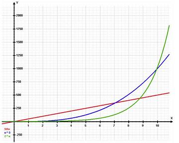
We want to know how TQ(N) grows as N grows. Quadratically, linearly? To answer this, we need more vocabulary. Let's say we have an ordinary function of N, call it f(N). f(N) could be anything. One example is:
Another might be:
We wish to compare the growth rate of TQ(N) with our mathematical function f(N). We say that
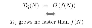
(The double array symbol, ⇔, means "if and only if".) We are giving our timing on algorithm Q an upper bound with the function f(N). In words, we say that "the timing for algorithm Q is Big-Oh of f(N)". The wording "grows no faster than" is not very rigorous, so we will make it air-tight using mathematical jargon.
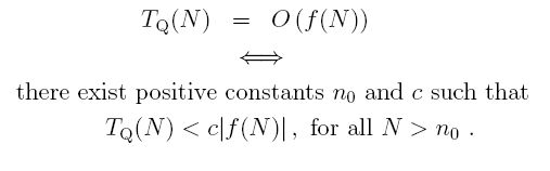
This means that while TQ(N) might start out being much greater than |f(N)| for small N, eventually, we are guaranteed that this will settle down as N increases and TQ(N) will never be greater than c|f(N )| for large N. (Since all our comparison functions, f(x) will be non-negative, I will drop the absolute value signs in many of the descriptions going forward.)
Linear Time, Logarithmic Time etc.
If TQ(N) is O(N) we say that Q is, at worst, a linear-time algorithm. It might actually be faster than linear, because this is only an upper bound. Here are the other commonly used bounding functions.
| f(N) | Informal Term for O(f(N)) |
|---|---|
| 1 | constant |
| logN | logarithmic |
| log2N | log-squared |
| N | linear |
| NlogN | (no special name) |
| N2 | quadratic |
| N3 | cubic |
| 2N | exponential |
You don't know what you think you know, so don't run out trying to sound smart just yet. That's because saying that algorithm is O(N2) doesn't necessarily mean that TQ(N) grows quadratically. All we have done is to provide an upper bound for the algorithm. O(N2) might be a sloppy and unnecessarily high upper bound. An algorithm Q that is O(N2) might also be O(N). Big-Oh is only an upper bound, it is not necessarily the exact growth rate of our algorithm. We will get to that.
Don't Worry About c
Some of you might get hung-up on the constant, c. Let's try to get over that now. Let's assume, for the sake of this demonstration, that if TQ(N) = cN (not <, but actually equals) for all large N. So we are assuming that algorithm Q is exactly linear, not just bounded by linear. It doesn't matter if c is large, like 100 or 1000. Remember, we're concerned with how the algorithm is sensitive to changes in N. If N doubles, what happens to TQ(N)? Well, if you are worried about c being 1000, let's see what happens if it is. That means that for large N we always know that TQ(N) = 1000N. What happens when we double N? Try it. The inequality assures us that TQ(2N) = 1000(2N). How much did the time increase? Take the ratio of the new time with the old one.
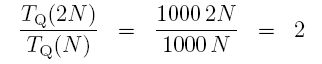
When N doubles, the time doubles. The constant, c, has nothing to do with the growth rate. So don't worry about it.
Now we can give the full mathematical definitions for the various growth rates.
As an exercise, to see if you understand this, take an algorithm (for fun, well call it R) and assume that R is quadratic (exactly, not just O(N2). Then, consider what happens when change the input size from N to 10N. That is, without knowing the c (but using it, because it must be used) compute how much longer the algorithm takes when you increase the array by a factor of 10. Hint: compute TR(10N) / TR(N).
3A.1.5 Ignoring the Small Stuff
You won't ever see anyone say that an algorithm is O(5N) or O(N2 + 9N). We would say, instead, that they are O(N) or O(N2). Why is that?
If an algorithm is O(5N) then it must also be O(N) -- the 5 does not add any information. The reason is that the 5 can be "absorbed" by the constant c in the definition of Big-Oh. The same reasoning, exactly, shows that O(3N2) is the same as O(N2). There is no point in ever having a constant factor in your Big-Oh.
Similarly, say that TQ(N) = O(N2 + 9N). This means that for large N:
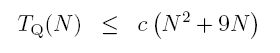
But for large enough N (N > 9, to be precise),
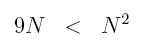
which means that for large N
Absorbing the 2 into the constant, c, we have just shown that
What we have demonstrated here is that, when discussing upper bounds on growth rates:
- only the highest power of N counts, and
- we never need a constant factor for the Np term.
The same logic that we used in the last section will show that if TQ(N) = O(f(N) + g(N)), and if f() grows faster than g(), we can "lose" the g(), i.e., TQ(N) = O(f(N)).
All of these observations will help us when computing growth rates, or time complexity, of algorithms.