Section 1 - Minimum Spanning Trees

11A.1.1 Early Congratulations

Welcome to week 11. If the car breaks down now, we can crawl home from here. So, congratulations - you've made it to the end of CS 2C, the third and final course in your C++-oriented computer science education. You are much more than a simple C++ programmer, now: you a computer scientist.

11A.1.2 The MST

The minimum spanning tree, or MST, is, roughly speaking, a sub-graph of any given graph that has all its unnecessary edges removed.

We're going to have to turn this into a class template and program, so I suppose you deserve something a little more precise than that, though.

Connectivity

We will assume that our graph is connected, that is, there is a path from every vertex to every other vertex. MSTs only apply to connected graphs. If the graph is not-connected, then we can take any connected components of it, and find the MST for that one connected component.

For example, we are interested in building a railway system on three continents. Clearly, there is going to be no rail track from a city on one continent to a city on another continent. We will have to apply the algorithm to one continent at a time. So we create a graph that connects every city in one continent to every other city in that same continent as a starting point. This will produce a graph that has three connected components, one for each continent. In order to produce an MST, we must consider the three connected components, individually.

Therefore, we lose no generality by assuming our input graph is connected.

Directedness

MSTs typically apply to non-directed graphs. For dijkstra, we represented non-directed graphs by storing both (v, w) and (w, v) in the adjacency table. For our MST algorithm, we can save time and space by placing either (v, w) or (w, v) in the graph, but not both. It won't matter which one we store, since the algorithm will treat the source and destination symmetrically (even though, the underlying graph data structure will have a different adjacency table if you use (v, w) than if you use (w, v)).

The Abstract Definition of MST

We return to our original description of a graph as being a collection of vertices, V, and a collection of edges, E. Each edge e in the set E consists of a pair of vertices (v, w) where v and w are both in the set V. Formally, we say G = {V, E }, i.e., it is determined by the two sets V and E.

An MST of a graph is going to be a new graph which has the same vertices as G, but whose edges are a subset of G's edges. Furthermore, the sum of all edge-costs in the sub-graph is as small as possible.

Minimum Spanning Tree

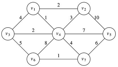
Often the idea is very simple, but the language needed for a formal definition is cumbersome. If you are not able to visualize the last definition, you should probably read it slowly with pencil and paper until you are. You can't get very far in a graduate program without being comfortable with this language. Here is picture of a graph, G, and its MST, G':

G

G' (MST of G)

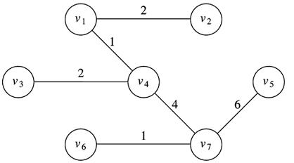
The picture embodies all the ideas of the abstract definition. G' has the exact same vertex set as G, but the edge set of G' is a subset of the edge set of G. Also, the MST remains connected. Finally, if you add the edge costs in G', it is as small as it can be. Try any other sub-tree of G and you'll get a larger total edge cost.

Observe that the final number of edges, |E'| is always one less than the number of vertices, |V| - 1.

Why the name "minimum spanning tree", and not "minimum spanning graph"? Certainly, the output is a graph, because we have done nothing to exclude it from that club. But not all graphs are trees. What makes it a tree?

The fact that you can choose a root (any node or vertex will do) and "pick up" the assemblage by that root, creating a cascade of children and grandchildren (or other descendents) from that node. It won't necessarily be a binary tree, but it will be a tree. If you tried this with the original graph, you would get "loops" connecting back up from some "grand children" to their "grand parents", distinct from the edges that took you from the "grand parent" down to the "grand children". It's kind of like the movies "Back to the Future" and "Hot Tub Time Machine".

This is a very imprecise explanation, but I'll make it more specific in the next section. For now, just notice that we may well be justified in calling this a "minimum spanning tree", and not a "minimum spanning graph".

11A.1.3 The Kruskal Algorithm

We will employ an algorithm by Kruskal, which, like dijkstra's algorithm, is very easy to describe. We'll do that in a moment. First, though, let's picture how we are going to implement it. Because an MST throws away edge data, it is important to preserve the original (input) graph. Therefore, we will have an external class for kruskal, which has as input an FHgraph object and which generates a second FHgraph object as a solution. The new graph should have the same vertices, but its adjacency table should be smaller.

Flipping the order of presentation, we will demonstrate the concept of having an external kruskal class and solution by listing the test client first, rather than last:

// FHkruskal client
// CS 2C Foothill College
#include <iostream>
#include <string>
using namespace std;
#include "FHgraph.h"
#include "FHkruskal.h"

// string is the data of the vertex; int is the cost type of edges
// --------------- main ---------------
int main()
{
   // build graph
   FHgraph<string, int> myGraph1, myGraph2;
   
   myGraph1.addEdge("v1","v2", 2);    myGraph1.addEdge("v1","v4", 1); 
   myGraph1.addEdge("v2","v4", 3);    myGraph1.addEdge("v2","v5", 10); 
   myGraph1.addEdge("v3","v1", 4);    myGraph1.addEdge("v3","v6", 5); 
   myGraph1.addEdge("v4","v3", 2);    myGraph1.addEdge("v4","v5", 7); 
   myGraph1.addEdge("v4","v6", 8);    myGraph1.addEdge("v4","v7", 4); 
   myGraph1.addEdge("v5","v7", 6); 
   myGraph1.addEdge("v7","v6", 1);

   myGraph1.showAdjTable();

   FHkruskal<string, int> kruskal(myGraph1);
   kruskal.genKruskal(myGraph2);

   cout << "ladies and gentlemen, ... I give you kruskal:" << endl;
   myGraph2.showAdjTable();

   return 0; 
}

What you see (two thirds of the way down the code) is the instantiation of a kruskal object with the input graph, myGraph1 as a constructor parameter After that, we retrieve the resultant MST for this input graph using the instance method genKruskal(), passing in a reference graph that will be modified to receive the MST result.

Although it is not pictured in this example, we can replace the input graph with a different graph after object instantiation using a simple mutator setInGraph().

This is one of many ways to represent the above-pictured non-directed graph. Here, is a successful test of kruskal's MST algorithm:

------------------------
Adj List for v1: v2(2) v4(1)
Adj List for v2: v4(3) v5(10)
Adj List for v4: v5(7) v3(2) v6(8) v7(4)
Adj List for v5: v7(6)
Adj List for v3: v1(4) v6(5)
Adj List for v6:
Adj List for v7: v6(1)

ladies and gentlemen, ... I give you kruskal:
------------------------
Adj List for v4: v7(4) v3(2)
Adj List for v7: v6(1)
Adj List for v6:
Adj List for v3:
Adj List for v2:
Adj List for v5: v7(6)
Adj List for v1: v4(1) v2(2)

Press any key to continue . . .

If you compare this run to the picture, you will confirm that it gives a correct MST.

Remember - in our regime, we will not distinguish between a directed and non-directed graph. This means that there are many different equivalent outputs. We will always get six edges, but the adjacency lists may be built differently, even using the same code on different machines. If you draw the pictures, they will all be the same.

Let's learn how the kruskal algorithm works and see how to code it.