Section 1 - The Dijkstra Algorithm

10B.1.1 A Shortest Path Algorithm: Dijkstra

We will use Dijkstra's algorithm for computing a shortest path. The problem is this: given a graph with only positive edge costs and a reference vertex, s, what is the shortest path from s to some other vertex, t?

To give an example, we use our familiar graph and ask the question "what is the shortest path from to v₂ to v₆?

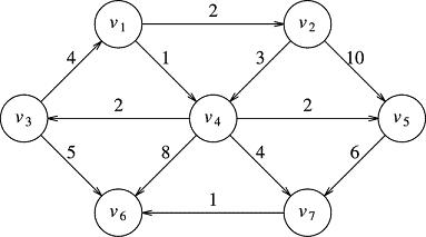
We can see numerous paths that will get us from to v₂ to v₆, but the algorithm must pick out the shortest and tell us the cost, or distance, of that shortest path. Here is the output from a successfully designed dijkstra algorithm:

Cost of shortest path from v2 to v6: 8.0
v2 -> v4 -> v7 -> v6

Breadth First

Dijkstra is called a breadth-first algorithm because it processes all the vertices adjacent to a given vertex, first, before going deeper. If there are four people standing around you, and you were looking for a friend somewhere else in the room, you would ask all four of them first, before deciding which way to go deeper into the crowd. The alternative is a depth-first algorithm in which you would ask only one of your neighbors and, following his suggestion, take a step in a certain direction until you are surrounded by four new neighbors. There you would again only ask one person and make a move deeper in. Once you had exhausted all of the leads, if you had not found your friend, you would return to your original starting point and ask the second of your original four neighbors. Dijksta takes the first approach. It processes all neighbors of a given vertex at each point in the algorithm.

To be slightly more precise, for a given vertex, v, we will process all of v's direct successors, first, before going deeper. A direct successor is simply a vertex on v's adjacency list, that is, a destination on an edge of which v is a source.

No Penalty for Computing All Shortest Paths from Vertex s.

While we may want to know the distance between two vertices, s and t, it turns out to be no faster to compute this shortest path than it does to compute the shortest path between s and all other vertices in the graph.

The Algorithm

The shortest path method we present now is a slight variant of the original Dijkstra algorithm. When implementing Dijkstra, there are various design choices that one can make which cause better performance in some graphs and poorer in others. There is no one implementation which is best for all. I have incorporated the specific choices directly into my basic algorithm here because it leads to a very simple and efficient algorithm, but the ideas are the same in all Dijkstra-like techniques. Afterward, we discuss how this differs from the purest form of Dijkstra and what you can do if you want to change variants.

Every vertex is thought of as having a distance value associated with it for the purposes of this algorithm. (This works out great for us, since we have already defined the FHvertex to contain an int member, dist, which we can use for just this purpose.) In the course of the algorithm, the distance associated with some vertex, w, will always be the cost of the some path from our reference vertex, s, to the vertex w. Our job is to get each vertex's distance to be the smallest it can be; it will ultimately represent the cost of the shortest path from s to w. As a side-effect, we will also store the shortest path from s to each vertex, w, as a list of edges or vertices that gets us from s to w using this smallest cost = shortest distance.

The algorithm is very easy to describe, but it takes some thinking to convince yourself it works. We will do both.

We initialize the distance from s to every vertex in the graph to be infinity (except for s, which has, of course, distance 0 to itself). To start the algorithm, "push" the first vertex, s, onto a stack, queue or set (we will use a queue, for reasons to be discussed shortly). This is the working queue of partially processed vertices. Now we go to work on that queue by "popping" a (any) vertex off of it. Call the "popped" vertex. v. We examine each of v's direct successors (ergo, breadth-first) in the following way: Say w is one of v's successors. If we can shorten w's distance from s to it using the path through v, then we replace the old distance stored in w with the new shorter distance through v and "push" that successor onto the queue of partially processed vertices. We continue until there are no more vertices on the queue. End of Algorithm.

Here is an outline of the algorithm.

That's the whole algorithm. When it's done, every vertex in the graph will have its distance value properly computed as the cost of the shortest path from s to it. The algorithm does not store any path information, but we will do so easily by adding one line in the code.

10B.1.2 Picturing Dijkstra

We begin by initializing all the vertices' distances, treating the reference vertex, s, as special:

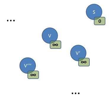
We "push" S onto our processing queue, as the first and only vertex. Then we begin an outer processing loop in which we "pop" one vertex off this queue for each loop pass, continuing until the queue is empty. Don't worry about the fact that there is only one vertex in the queue to start. We will "push" more during the first loop pass.

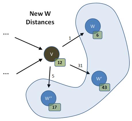
Let's describe a typical pass of this outer loop. It begins by "popping" a vertex off the queue:

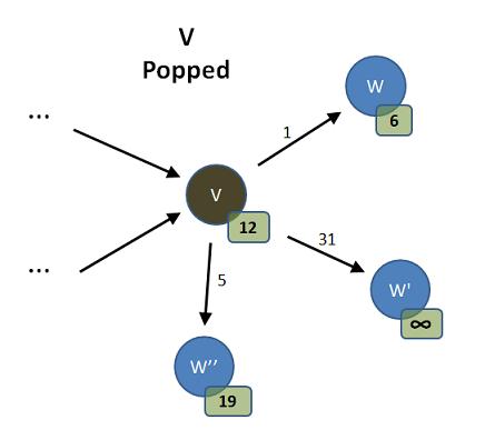
We show a vertex, V, "popped"; it is no longer in the queue, but we have it, locally, and will process it in this outer loop pass. We also see V's immediate successors. We picture them as the Ws in the diagram above. They are the vertices to which V points - the members of V's adjacency list. We also show hypothetical distance values for V and its neighbors. These are the distances computed, so far, from our reference S to that vertex. Also, we show the cost of the edges that take us from V to each W. This, then is the picture as we begin the next pass of our outer loop.

Dijkstra tell us we should enter an inner loop that processes all the vertices in V's adjacency list - the Ws. We will iterate through this adjacency list and ask the question of each W we find, "If I pass through V to get to W, will I lessen W's distance (to S)?" Here are the answers to this question for the picture above:

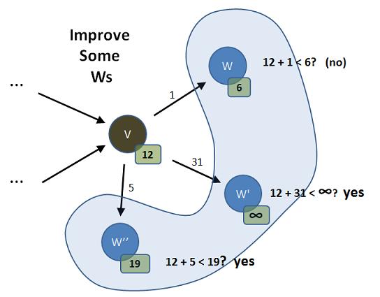
This shows us that two of the Ws can be improved by going through V: W' and W''. The other one, W, is better using whatever path it had calculated in earlier passes of the outer loop. Dijkstra tells us that we should update the distances where they make things better (i.e., shorter):

Finally, we "push" the improved Ws onto the queue and do nothing for the Ws that are not improved:

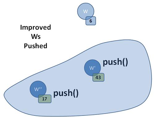
This completes a pass of the outer loop. As you see, it is only making distances shorter, never larger. The claim is that when the queue is empty, all distances are at their minimum. We'll want to examine this claim next, and talk about the choice of a queue (vs. set, priority_queue or stack) as the container to hold the collection of partially processed vertices.