Section 1 - Motivating the Graph

10A.1.1 Three Shortest Path Problems

Graph theory and its algorithms are unlike all the previous data structures and algorithms we have studied so far. Because this field addresses such a loosely knit collection of problems, each of which is just different enough from the others to warrant a disparate approach to its solution, there are no standard graph libraries or algorithm packages that are of practical use to programmers. One has to analyze and then program each problem by hand. That doesn't mean that we cannot collect a coherent tool set that can be reused. It merely means that the tools tend to be in the form of abstract algorithms and pseudo-code rather than ready-made software libraries, classes or container templates.

This week and next we are going to try to buck this bleak reality and go one step beyond what most texts and articles provide. We will actually attempt to provide a couple C++ template classes for graphs that can at least be a starting point for future C++ work. If nothing else, the analysis of how this real code is created -- from theory to execution -- will be a model that you can refer back to when attacking your own future graph problems.

We begin by looking at three problems that have a common theme, and then abstracting the common features of each. This contrasts the usual approach of defining a graph first and later showing applications. The advantage of our approach is that graph-theoretical definitions are incredibly boring and hard to memorize in a vacuum, but if you have a problem in mind before-hand, the definitions seem so natural that their memorization is painless.

10A.1.2 Wide Area Networks (WANs)

Consider a collection of computers around the world that are connected by a network. This isn't hard to imagine - you are reading this page on one such network. Every time you follow a link, you are connected to a distant computer through a series of intermediate computers, called routers. Typically, you have a dozen or so such routers through which information has to travel in order to get from the device your fingers are touching and the source of the text, graphic or video that you are studying. Here is an example of the route taken between my cabin on the Olympic Peninsula in Washington state and some computer in Amsterdam. It starts in Amsterdam:

1 new51-new50-racc1.new.seabone.net (195.22.216.195)
2 be-10-204-pe01.111eighthave.ny.ibone.comcast.net (75.149.230.77)
3 pos-1-9-0-0-cr01.newyork.ny.ibone.comcast.net (68.86.86.41)
4 pos-2-11-0-0-cr01.chicago.il.ibone.comcast.net (68.86.86.234)
5 pos-1-12-0-0-cr01.denver.co.ibone.comcast.net (68.86.85.250)
6 pos-0-14-0-0-cr01.seattle.wa.ibone.comcast.net (68.86.85.209)
7 pos-0-15-0-0-ar01.seattle.wa.seattle.comcast.net (68.86.90.214)
8 be-30-ar01.burien.wa.seattle.comcast.net (68.85.240.70)
9 te-9-1-ur01.bremerton.wa.seattle.comcast.net (68.86.96.45)
10 ge-4-0-0-ten01.bremerton.wa.seattle.comcast.net (68.87.205.42)

I cut off the last two computers to protect my privacy, but you can see that it took 10 computer routers to pass the signal from Amsterdam to my local provider at the cabin, the first one being a router in Italy, and from there to New York, Chicago, Denver, Seattle, etc. Starting at the same computer in Amsterdam, and requesting a ping to Stanford University, we get the following set of routers in the path:

1 fra32-fra52-racc2.fra.seabone.net (89.221.34.107)
fra32-fra18-racc1.fra.seabone.net (89.221.34.53)
fra32-fra52-racc2.fra.seabone.net (89.221.34.107)
2 te7-3.mpd02.fra03.atlas.cogentco.com (130.117.15.45)
3 te7-7.mpd02.par01.atlas.cogentco.com (130.117.1.242)
4 te7-7.mpd02.lon01.atlas.cogentco.com (130.117.2.6)
te7-3.ccr01.par04.atlas.cogentco.com (130.117.2.78)
te7-7.mpd02.lon01.atlas.cogentco.com (130.117.2.6)
5 te7-4.mpd03.jfk02.atlas.cogentco.com (130.117.1.105)
te9-2.ccr04.jfk02.atlas.cogentco.com (154.54.0.209)
6 te1-8.mpd01.ord01.atlas.cogentco.com (154.54.29.157)
7 te0-4-0-0.ccr22.mci01.atlas.cogentco.com (66.28.4.33)
te0-1-0-2.mpd21.mci01.atlas.cogentco.com (66.28.4.185)
8 te9-4.mpd01.sfo01.atlas.cogentco.com (154.54.2.210)
te7-4.ccr02.sfo01.atlas.cogentco.com (154.54.5.198)
te2-2.ccr02.sfo01.atlas.cogentco.com (154.54.6.42)
9 te7-4.mpd01.sjc04.atlas.cogentco.com (154.54.28.82)
10 Stanford_University2.demarc.cogentco.com (66.250.7.138)
11 boundarya-rtr.Stanford.EDU (68.65.168.33)

This time, it went first to Frankfort, Germany, then France, then a number of computers until it gets to San Jose and finally Stanford.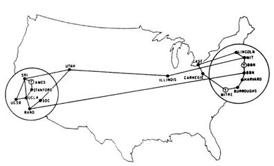

How are these paths determined? There are millions of ways to get from Amsterdam to my cabin, and millions more that get you from Amsterdam to Stanford. Yet if you perform these so-called "trace routes" many times, you will get almost identical paths to each time. Somehow, somewhere, there is a software algorithm that is finding the shortest (or maybe fastest) route from one "vertex" (a computer) in Amsterdam to another "vertex" (a computer in Washington or California).

You can picture the network of computer routers as a collection of dots or "vertices" connected by fiber optic cables to each other. The cables are sometimes called "edges". Not every two routers 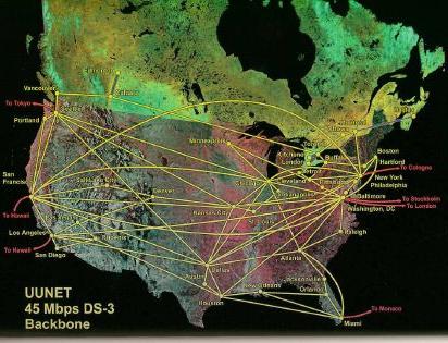are directly connected, but you can usually find a "path" from one router to another through a series of intermediate routers. We, of course, want the shortest path.

In this picture, all the edges are shown as simple lines, but there is an additional piece of information that goes along with those lines. It is implied by the picture. Can you guess what it is?

The implied information is each line's length. Symbolically, if two routers (vertices) are farther apart, their lengths are longer and this implies a longer travel time (because signals do take longer to go long distances than they do to go short distances, even if they are travelling at the speed of light). You can then imagine attached to each edge, a number that would represent the length -- or "distance" or "cost" -- of that edge in the computer network. So ... we have routers (the vertices). We have fiber optic cables (the edges). And we have distances (or costs) for each edge. The problem that must be solved is, given any two routers (vertices), find the shortest path (a collection of edges whose total cost is the smallest). This is the famous shortest path problem.

10A.1.3 Flight Reservations

This last picture looks like it might also represent actual travel from one city to another by air travel. Let's switch over to that problem, now. You are writing software for a travel site and the problem is to compute all the reasonable (i.e., shortest) paths from one origin city to the destination city. Here is what the user enters:

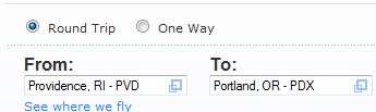
and here is what your program will display:

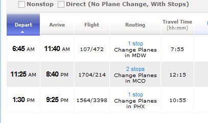
Of all the hundreds of ways to fly from Providence, RI, to Portland, OR, the program found three. Two had one stop, and one had two stops. There may have been dozens with only one stop, but the flight with two stops beat most of them out. Why? Cost (distance). Not only does the fewest number of intermediate stops matter, but so does the cost of the flights in terms of distance and time. Here we have a similar picture. Each city or airport is a vertex. The flights form edges. And the cost of each edge is the distance between cities. The problem, again, is to compute the shortest path.

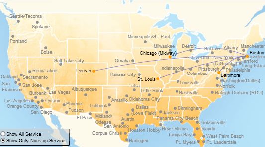
To give you an idea of the difficulty, here is the small set of flights that directly connect Providence, RI to destinations. There are only four.

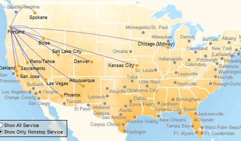
Meanwhile, here are the non-stops to/from Portland:

The program found two paths you can deduce from these two pictures, but one that didn't appear on either. It did so by considering dozens of maps, each of which contains dozens of paths like this one, centered at San Antonio:

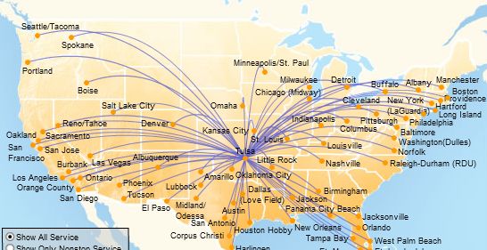
If we tried to show the flights between every two cities on the same map, it would be too dense to read. The idea is simple, though. We want to consider all the edges (routes) between all the vertices (cities) and find the ones with the least cost.

10A.1.4 Computer Games and Process Simulation

In programs that simulate reality, especially those that play computer and video games, there is always an internal game "state". The state represents the condition of the board or universe at any point in time. For example, the state may include the information that

• your player has a shield operating at half strength,
• your player has six allies, and
• your player is standing three feet from an adversary.

How you got into that state is not important, but if you are hit with a laser, this state determines what your next state will be. If the laser hits your shield, it may reduce the shield to 1/3 strength and you may fall back four feet from the adversary. This is your new state .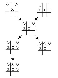

Each state in a computer game can also be called a node or vertex. There are only a finite number of states you can get to from your current state, and each of these can be thought of as connected to it by an edge. The edge would represent an action that could take you from one state to the next. Again, being hit by a laser might be part of the description of an edge between your current state (shield power = .5) and your subsequent state (shield power = .33).

We can use vertices and edges to represent legal moves in a game of tic-tac-toe. You can see the states (vertices) and possible moves (edges) in the adjacent diagram. Just like in the case of network routers or flights between cities, there are only certain states that are directly reachable from any given state.

This example covers more than games. A construction project, a Fedex order-tracking problem or any large scale effort that has a number of intermediate phases can be represented by states and the transitions (edges) between them.

In many simulations, games or otherwise, it is important for the computer to determine the shortest path between two states. This is the same problem, conceptually, as the first two we considered -- the shortest path problem.

10A.1.5 Directed and Non-Directed Edges

One difference between the game example and the previous two appears to be that, in games, the edges are directed: You cannot erase an X in a tic-tac-toe board to back up to a previous state. However, you can fly between two cities in either direction (and send signals between routers in either direction). However, this difference is illusory. In truth, the edges between cities may seem non-directional only because we are clumping two directed edges in our minds into one non-directed edge. That is, we did not distinguish between the flight from Providence to Chicago and the flight back from Chicago to Providence. We assumed that both flights represented the same connection. However, rather than one non-directed edge between these two cities, in reality, we have two directed edges between Providence and Chicago, one that goes east and one that goes west. Same with routers. While the fiber optic cable appears to be bi-directional, we really have separate receive and send pathways and it is possible to disable one direction without disabling the other. Again, a single non-directed edge between two routers:

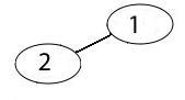
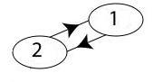
can be more accurately represented by two directed edges, one pointing from router 1-to-2 and another pointing from 2-to-1:

10A.1.6 The Graph Abstraction

I think you are starting to get the idea. There is a similarity between all these problems. The first connection is the data itself. We are using objects called nodes or vertices (singular vertex) and connections between the two called edges. An edge can be directed (it points from one vertex to another) or non-directed (there are no arrows at all, which we could equate to two arrows if we wish). The second connection is the problem to be solved: We are interested in the shortest path between two vertices.

Here is how we will abstract, graphically, the notions of vertices and edges into a data structure we will call a graph.

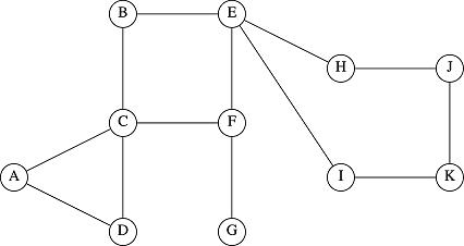
This graph consists of vertices which are represented by letters, A, B, C, ... and stand for the actual objects in a particular graph. They might be cities, computer routers or game states. It doesn't really matter, from the point of view of the graph algorithm, what that vertex is. What does matter is the topology, i.e., to what vertices do these edges attach? In other words, once you draw the graph like this, you can work with only the edges and vertices to find a shortest path.

The above graph had non-directional edges and was therefore called an undirected graph. A graph whose edges are directed are represented with arrows between the vertices:

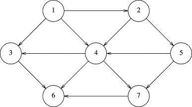
Here, we can get from vertex 1 to vertex 4, but we cannot get from 4 to 1. In fact, we cannot get from any vertex 2 or higher back to 1. Also, if we start at vertex 6, we are "done". There is nowhere to go from there. A directed graph is sometimes shortened to digraph.

The one ingredient that we are missing is the cost of each edge. Normally, all edges are not created equal. It might be that you can get from San Francisco to Dallas using a path with only one stop (two edges), but that stop might be New York! Meanwhile there may be a route that gets you from San Francisco to Dallas in two stops (three edges) that go through LA and Phoenix, but that route is shorter and faster. We need to know the cost of each edge. Here is how we represent the costs of the edges:

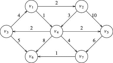
This gives us all the information we need to solve almost any problem involving the graph. Let me finish this page by saying that the shortest path problem, while important, is only one of hundreds of problems in graph theory. We will now consider a second big issue: the minimum spanning tree.